Gaussian Mixture Models
Gaussian Mixtures
A Gaussian mixture model is a probabilistic model that assumes all the data points are generated from a mixtures of a finite number of Gaussian distributions with unknown parameters.
One can think of mixture models as generalizing k-means clustering to incorporate information about the covariance structure of the data as well as the centers of the latent Gaussians.
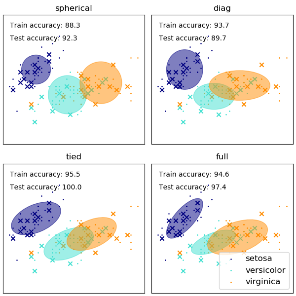
Sklearn’s GaussianMixture comes with different options to constrain the covariance of different classes estimated, as shown in this picture:
Example
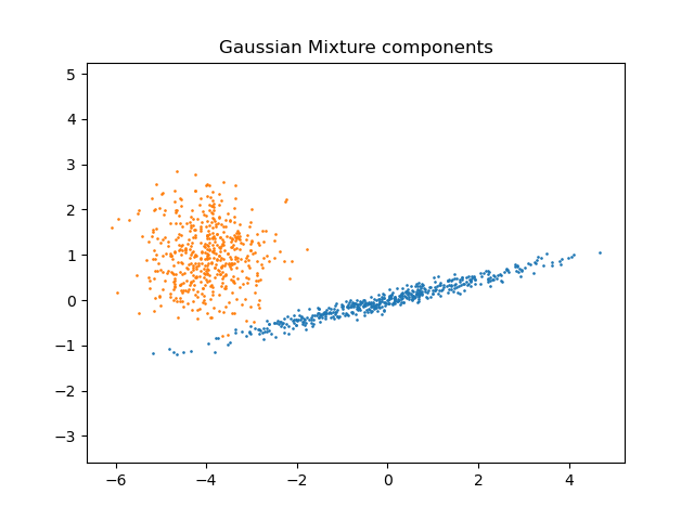
See the example Gaussian Model Selection
1
2
3
4
5
6
7
8
9
10
11
12
13
14
15
16
17
18
19
20
21
22
23
24
25
26
27
28
29
30
31
32
33
34
35
36
37
38
39
40
41
42
43
44
45
46
47
48
49
50
51
52
53
54
55
56
57
58
59
60
61
62
63
64
65
66
67
68
69
70
71
72
73
74
75
76
77
78
79
80
81
82
import numpy as np
import itertools

from scipy import linalg
import matplotlib.pyplot as plt
import matplotlib as mpl

from sklearn import mixture

print(__doc__)

# Number of samples per component
n_samples = 500

# Generate random sample, two components
np.random.seed(0)
C = np.array([[0., -0.1], [1.7, .4]])
X = np.r_[np.dot(np.random.randn(n_samples, 2), C),
          .7 * np.random.randn(n_samples, 2) + np.array([-6, 3])]

lowest_bic = np.infty
bic = []
n_components_range = range(1, 7)
cv_types = ['spherical', 'tied', 'diag', 'full']
for cv_type in cv_types:
    for n_components in n_components_range:
        # Fit a Gaussian mixture with EM
        gmm = mixture.GaussianMixture(n_components=n_components,
                                      covariance_type=cv_type)
        gmm.fit(X)
        bic.append(gmm.bic(X))
        if bic[-1] < lowest_bic:
            lowest_bic = bic[-1]
            best_gmm = gmm

bic = np.array(bic)
color_iter = itertools.cycle(['navy', 'turquoise', 'cornflowerblue',
                              'darkorange'])
clf = best_gmm
bars = []

# Plot the BIC scores
plt.figure(figsize=(8, 6))
spl = plt.subplot(2, 1, 1)
for i, (cv_type, color) in enumerate(zip(cv_types, color_iter)):
    xpos = np.array(n_components_range) + .2 * (i - 2)
    bars.append(plt.bar(xpos, bic[i * len(n_components_range):
                                  (i + 1) * len(n_components_range)],
                        width=.2, color=color))
plt.xticks(n_components_range)
plt.ylim([bic.min() * 1.01 - .01 * bic.max(), bic.max()])
plt.title('BIC score per model')
xpos = np.mod(bic.argmin(), len(n_components_range)) + .65 +\
    .2 * np.floor(bic.argmin() / len(n_components_range))
plt.text(xpos, bic.min() * 0.97 + .03 * bic.max(), '*', fontsize=14)
spl.set_xlabel('Number of components')
spl.legend([b[0] for b in bars], cv_types)

# Plot the winner
splot = plt.subplot(2, 1, 2)
Y_ = clf.predict(X)
for i, (mean, cov, color) in enumerate(zip(clf.means_, clf.covariances_,
                                           color_iter)):
    v, w = linalg.eigh(cov)
    if not np.any(Y_ == i):
        continue
    plt.scatter(X[Y_ == i, 0], X[Y_ == i, 1], .8, color=color)

    # Plot an ellipse to show the Gaussian component
    angle = np.arctan2(w[0][1], w[0][0])
    angle = 180. * angle / np.pi  # convert to degrees
    v = 2. * np.sqrt(2.) * np.sqrt(v)
    ell = mpl.patches.Ellipse(mean, v[0], v[1], 180. + angle, color=color)
    ell.set_clip_box(splot.bbox)
    ell.set_alpha(.5)
    splot.add_artist(ell)

plt.xticks(())
plt.yticks(())
plt.title('Selected GMM: full model, 2 components')
plt.subplots_adjust(hspace=.35, bottom=.02)
plt.show()
Key Takeaways
For model selection in GMM, BIC is better suited because of the information derived both from covariance type as well as number of components: