Get Pandas Datareader
ProTip: Be sure to remove /docs and /test if you forked Minimal Mistakes. These folders contain documentation and test pages for the theme and you probably don’t want them littering up your repo.
1
2
3
| import pandas as pd
import numpy as np
from pandas_datareader import data
|
Get Google stock prices
1
2
| goog = data.DataReader('GOOG', start='2004', end='2018', data_source='yahoo')
goog.head()
|
|
High |
Low |
Open |
Close |
Volume |
Adj Close |
| Date |
|
|
|
|
|
|
| 2004-08-19 |
51.835709 |
47.800831 |
49.813286 |
49.982655 |
44871300.0 |
49.982655 |
| 2004-08-20 |
54.336334 |
50.062355 |
50.316402 |
53.952770 |
22942800.0 |
53.952770 |
| 2004-08-23 |
56.528118 |
54.321388 |
55.168217 |
54.495735 |
18342800.0 |
54.495735 |
| 2004-08-24 |
55.591629 |
51.591621 |
55.412300 |
52.239193 |
15319700.0 |
52.239193 |
| 2004-08-25 |
53.798351 |
51.746044 |
52.284027 |
52.802086 |
9232100.0 |
52.802086 |
1
| goog_p = goog['Adj Close']
|
1
2
3
4
| %matplotlib inline
import matplotlib.pyplot as plt
plt.style.use('seaborn-ticks')
import seaborn; seaborn.set_style('whitegrid')
|
1
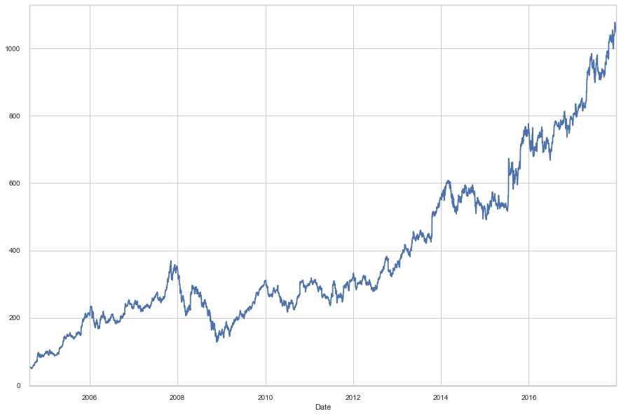
| goog_p.plot(figsize=(15,10))
|
1
| <matplotlib.axes._subplots.AxesSubplot at 0x128dc0610>
|
Compute Yearly Return
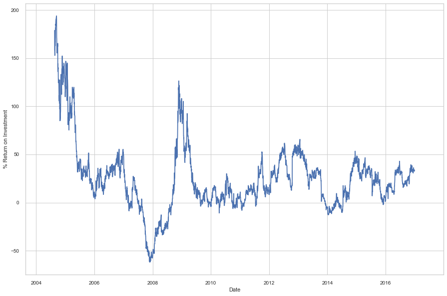
A common context for financial timeseries data is computing difference over time. For example, we can calculate one-year returns using pandas.
1
2
3
4
5
| goog_p = goog_p.asfreq('D', method='pad')
ROI = 100 * (goog_p.tshift(-365)/goog_p - 1)
ROI.plot(figsize=(15, 10))
plt.ylabel('% Return on Investment');
|
1
2
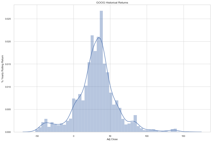
| y1_return = goog['Adj Close'].pct_change().rolling(365).sum().dropna()
y1_vol = goog['Adj Close'].pct_change().rolling(365).std().dropna()
|
1
2
3
4
| plt.figure(figsize=(15, 10))
seaborn.distplot(y1_return*100)
plt.ylabel('% Yearly Rolling Return')
plt.title('GOOG Historical Returns');
|