NIFTY Index Performance
NIFTY Index Performance
Here are some of the key insights from the chart and summary statistics:
| Period | Mean | Median | Min | Max | Std Dev |
|---|---|---|---|---|---|
| 10 Year | 10.88 | 11.30 | 4.04 | 16.56 | 2.56 |
| 15 Year | 9.47 | 9.44 | 7.47 | 12.13 | 1.34 |
| 5 Year | 10.74 | 11.72 | -3.20 | 21.06 | 4.19 |
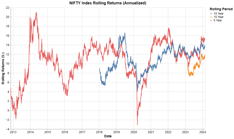
Conclusion
The NIFTY Index has shown significant growth over the years, with clear upward trend in the last 10 years as we are in a bull market.
1
2
3
4
5
6
7
8
9
10
11
12
13
14
15
16
17
18
19
20
21
22
23
24
25
26
27
28
29
30
31
32
33
34
35
36
37
38
39
40
41
42
43
44
45
46
47
48
49
50
51
52
53
54
55
56
57
58
59
60
61
62
63
64
65
66
67
68
69
70
71
72
73
74
75
76
77
78
79
80
81
82
83
84
85
86
87
88
89
import pandas as pd
import yfinance as yf
import altair as alt
import numpy as np

# Download NIFTY data (using ^NSEI ticker)
nifty = yf.download('^NSEI', start='1999-01-01', end='2024-02-22')

# Ensure we have the Adj Close column and calculate daily returns
if 'Adj Close' not in nifty.columns:
    nifty['Adj Close'] = nifty['Close']
nifty['Daily_Return'] = nifty['Adj Close'].pct_change()

# Function to calculate rolling returns (annualized)
def calculate_rolling_returns(data, years):
    rolling_periods = years * 252  # Using 252 trading days per year
    rolling_returns = (1 + data['Daily_Return']).rolling(window=rolling_periods).apply(
        lambda x: np.prod(x)) ** (252/rolling_periods) - 1
    return rolling_returns * 100  # Convert to percentage

# Create an empty DataFrame for rolling returns
rolling_returns_df = pd.DataFrame()
rolling_returns_df.index = nifty.index

# Calculate different rolling returns
periods = [5, 10, 15, 20]
for period in periods:
    col_name = f'{period}Y_Rolling'
    rolling_returns_df[col_name] = calculate_rolling_returns(nifty, period)

# Reset index to make date a column
rolling_returns_df = rolling_returns_df.reset_index(drop=False)

# Melt the dataframe for Altair plotting
rolling_returns = pd.melt(
    rolling_returns_df,
    id_vars=['Date'],
    value_vars=[f'{period}Y_Rolling' for period in periods],
    var_name='Period',
    value_name='Return'
)

# Clean up period names for display
period_mapping = {f'{period}Y_Rolling': f'{period} Year' for period in periods}
rolling_returns['Period'] = rolling_returns['Period'].map(period_mapping)

# Remove any NaN values
rolling_returns = rolling_returns.dropna()

# Create Altair chart
chart = alt.Chart(rolling_returns).mark_line().encode(
    x=alt.X('Date:T', title='Date'),
    y=alt.Y('Return:Q',
            title='Rolling Returns (%)',
            scale=alt.Scale(zero=False)),
    color=alt.Color('Period:N', title='Rolling Period'),
    tooltip=[
        alt.Tooltip('Date:T', title='Date'),
        alt.Tooltip('Return:Q', title='Return (%)', format='.2f'),
        alt.Tooltip('Period:N', title='Period')
    ]
).properties(
    width=800,
    height=500,
    title='NIFTY Index Rolling Returns (Annualized)'
).configure_axis(
    labelFontSize=12,
    titleFontSize=14
).configure_title(
    fontSize=16
).configure_legend(
    labelFontSize=12,
    titleFontSize=14
)

# Display the chart
chart

# Calculate summary statistics
summary_stats = rolling_returns.groupby('Period')['Return'].agg([
    ('Mean', 'mean'),
    ('Median', 'median'),
    ('Min', 'min'),
    ('Max', 'max'),
    ('Std Dev', 'std')
]).round(2)

print("\nSummary Statistics of Rolling Returns:")
print(summary_stats)